Introduction

Over the past decade, generative models have advanced significantly. Initially capable of simple tasks like generating digits (0–9), they have progressed to sophisticated capabilities, such as creating a wide range of realistic images of humans and animals, and imaginative depictions like hybrid human-animal forms and beyond. In 2014, Ian Goodfellow introduced Generative Adversarial Networks (GANs), featuring the architecture illustrated in Figure 1. Imagine two artists in a competition. One, called the “generator,” creates fake art, like counterfeit money. The other, the “discriminator,” tries to distinguish fake art from real art. The generator keeps improving its fakes to fool the discriminator, while the discriminator gets better at catching fakes. This competition continues until the generator makes art that’s so good, that the discriminator can’t tell the difference. In the end, you get incredibly realistic fake art that can even resemble Hollywood celebrity faces shown in Figure 1 below.

Furthermore, another research gained attention in early 2014, Variational Autoencoders (VAEs) for synthesizing images.

A Variational Autoencoder (VAE) works like this:

1. Input Data: We start with input data, like images.

2. Encoder: The Encoder compresses the input data into a smaller, simpler representation, called the “latent space.”

3. Latent Space: The latent space is a condensed version of the input data, capturing its most important features.

4. Decoder: The Decoder takes this compressed representation and tries to reconstruct the original input data from it.

5. Output (Reconstruction): The goal is for the Decoder to recreate the input data as accurately as possible from the latent space.

6. Variational Part: The VAE adds some randomness (noise) to the latent space to make the model better at generating new, similar data.

In short, a VAE learns to compress data into a simpler form and then reconstruct it, adding a bit of randomness to create new, similar data.

Finally, Diffusion Models came in 2021 that revolutionised the process of generating images. The model used in DALLE-2, the previous version being DALLE, uses a variant of a transformer model, similar to the architecture used in GPT-3.

Let’s understand how the data is synthesised

In machine learning, we assume that all data such as images, audio, videos, text, and so on comes from a distribution. The goal of the generative model is to learn this distribution and seek samples from it that get other data points that look like they come from the training dataset.

For instance:

In the above example, the model learns from the training set and generates an almost similar sample in the test set. This distribution is not known to us, we learn this data sample by ourselves. However, how do we learn this distribution?

Methods for Learning a Distribution

1. Likelihood-Based Approach: This method defines the distribution through its likelihood. The high value of likelihood for a sample definitely means that the sample is likely from the distribution. This will maximize the likelihood of generated samples and improve the model in matching the target distribution.

2. Divergence Minimization Approach: This method minimizes the difference (divergence) between the real data distribution and the model’s learned distribution. It is conventionally utilized in generative models to ensure the model represents an extremely close representation of the true distribution of the data.

Generating Samples from Learned Distribution

Once the model has learned the data distribution, we generate new samples (like images) from this distribution.

• GANs: Use a latent noise vector fed into a generator to produce an image.
• VAEs: Transform random noise through the model to generate an image.

Both methods involve a single step to create the final image.

Diffusion Models

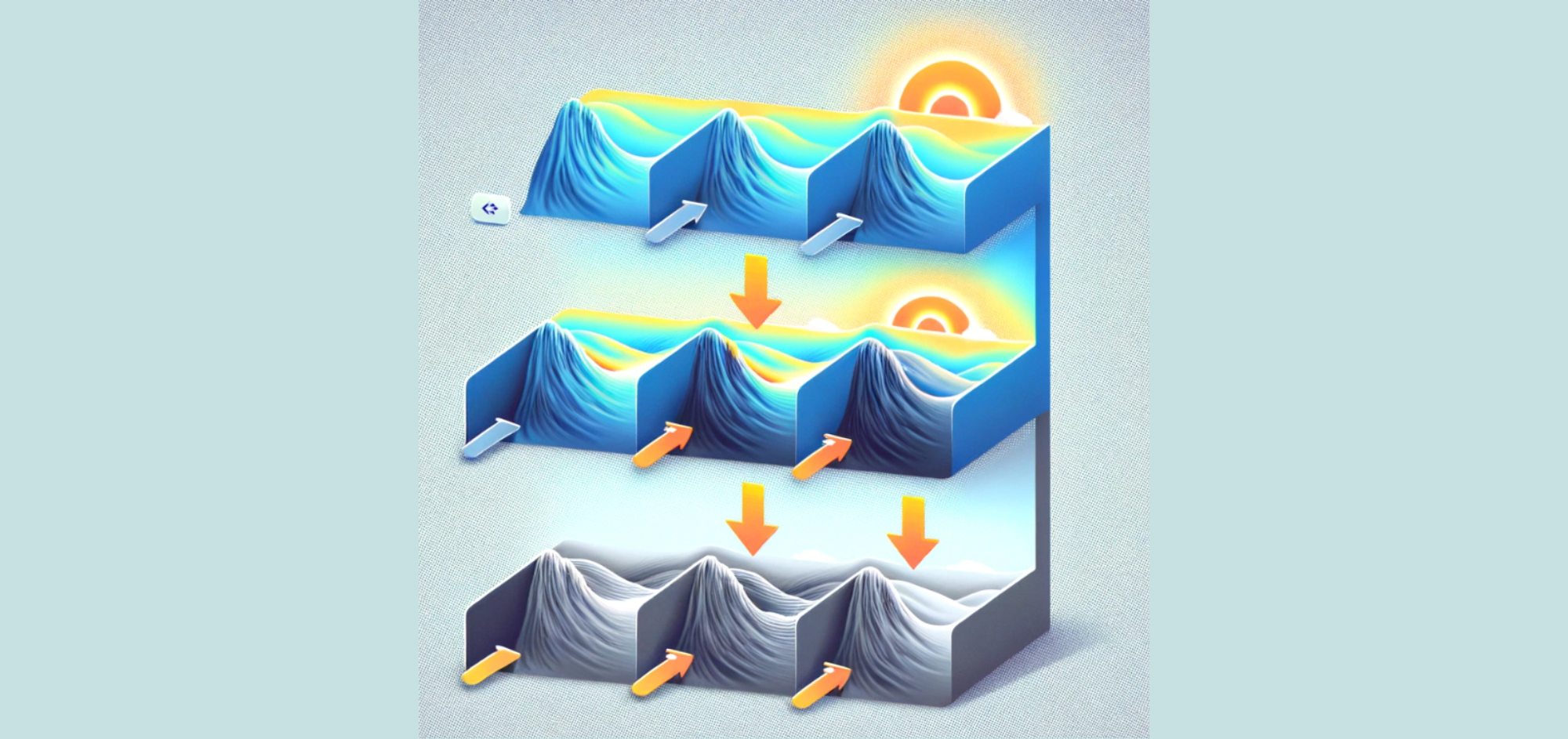
A diffusion model begins with a clean image that is progressively cluttered with noise to appear increasingly random. From a totally noisy image, it then learns how to reverse this process, gradually eliminating the noise to produce a new, clear image.

• Instead of one large step, they take multiple tiny steps using a Markov chain, making the process easier to analyse.
• Each step gradually refines the noise into a realistic image.

A Markov chain is a mathematical system that transitions from one state to another within a finite state space, and it is used here to iteratively refine the image from noise. For a deeper understanding, you can read more about Markov chains here.

Diffusion models have two steps:

1. Forward Process:

Take a datapoint x0 and gradually add very small amounts of Gaussian noise to it

• Let xt be the datapoint after t iterations
• This is called the forward diffusion process
• Repeat this process for T steps — over time, more and more features of the original input are destroyed until you get something resembling pure noise

More formally, we update each image over time as

Where,

is called the noise schedule (basically a hyperparameter describing “how much” noise to add at a given timestep). The update above can equivalently be written as a sampling process from the following Gaussian distribution:

In simple terms,

• This process gradually adds noise to an image using a sequence of Markov chain steps.
• Each step is simple and predefined, progressively degrading the image quality until it becomes pure noise.

2. Reverse Process:

The goal of a diffusion model is to learn the reverse denoising process to iteratively undo the forward process. That is, to generate the original noise-free image.

In this way, the reverse process appears as if it is generating new data from random noise. However, generating an image from noise is very hard and is not computationally tractable.

Why is 𝑞(𝑥𝑡−1∣𝑥𝑡) Unknown?

• Forward Process: In the forward process, we define how noise is added (from 𝑥0 to 𝑥𝑇​), so we know 𝑞(𝑥𝑡∣𝑥𝑡−1).
• Reverse Process: In the reverse process, we want to know 𝑞(𝑥𝑡−1∣𝑥𝑡), which is the probability distribution of the previous step given the current noisy data. This is much harder because we need to infer how to remove noise at each step, and the exact reverse distribution is not directly available.
• For instance: Take, for example, a clear picture that you gradually add a little blur to until it is totally unrecognizable and blurry. This is like the forward process.
• Now, you want to get back to the original clear photograph. You start with a completely blurry image and try to remove the blur little by little. However, you don’t know exactly how much blur was added at each step, so it’s challenging to perfectly undo the blurring process. This is the reverse process. The goal of the diffusion model is to learn how to remove the blur step by step to recover the original clear photograph.

Model’s Role

The role of the diffusion model is to approximate this unknown distribution 𝑞(𝑥𝑡∣𝑥𝑡−1) using a neural network that learns to predict and remove the noise. During training, the model learns from examples of noisy and clean images to get better at making these predictions.

Let’s understand in detail how this neural network works in the diffusion model:

Forward Process (Algorithm 1: Training Phase)

1. Adding Noise: We start with a clean data point 𝑥0. We add noise in multiple steps to generate noisy versions 𝑥1, 𝑥2,…..,𝑥𝑇​.

· This process is defined by the equations in the forward process, where noise is added in a controlled manner.

2. Training the Neural Network:

· Input: The neural network takes a noisy data point 𝑥𝑡 at a given time step 𝑡 and the time step 𝑡 itself as inputs.

· Output: The network predicts the noise 𝜖𝜃 (𝑥𝑡, 𝑡) that was added in step 5.

· Objective: The goal is to minimize the difference between the predicted noise and the actual noise added during the forward process.

Reverse Process (Algorithm 2: Sampling Phase)

1. Starting with Noise: We start with a data point that is pure noise 𝑥𝑇​.

2. Iterative Denoising:

• Step-by-Step Denoising: For each time step from 𝑇 down to 1, we use the neural network to predict the noise that needs to be removed.
• Update Equation: Using the predicted noise, we update the data point to remove some of the noise, progressively making it less noisy and more like the original clean data.
• The updated equation is:

Here, 𝜖𝜃 (𝑥𝑡, 𝑡) is the noise predicted by the neural network, and 𝑧 is additional noise added for stability.

3. Final Output: After iterating through all the steps, the final data point 𝑥0 should be a clean version that resembles the training data.

Image Generation using U-Net

Image Generation with U-Net, Attention, and ResNet Blocks:

• U-Net: A neural network that consists of an encoder and decoder. From a latent representation that the encoder compresses, the decoder reconstructs the image. With this arrangement, the model can record and make use of fine features at several scales.
• ResNet Blocks: These blocks are included in the U-Net so that, through skip connections, deeper networks may be trained. Training stability and learning efficiency are increased by this easier gradient flow during training.
• Attention Mechanisms: By better-capturing dependencies and details, attention mechanisms allow the model to concentrate on key areas of the image, enhancing its capacity to produce high-quality images.
• Integration in Diffusion Models: These elements are used to iteratively eliminate noise from the noisy latent representation, producing high-quality images, an opposite procedure to the forward process of diffusion models.

Further Trick for Enhancing Image Generation

Linear Vs Cosine Schedule

In above Figure Linear (Top), A linear noise schedule converts initial data to noise really quickly, making the reverse process harder for the model to learn.

Researchers hypothesized that a cosine-like function that is changing relatively gradually near the endpoints might work better.

Classifier Free Guidance

Classifier-free guidance is the preferred method in diffusion models to make image creation easier. Traditionally, Classifier Guidance enhances the quality and relevance of images produced by the model using a separate classifier. But this guiding mechanism is included straight into the diffusion model with Classifier-Free Guidance. It can successfully direct the image-generating process towards a particular class without the need for an additional classifier by training the model with and without class information. This results in a simpler and more effective model that nevertheless produces excellent, class-specific images.

Results

Diffusion Beats GANs

The above result looks very similar. However, if you see the left side of the result of BigGAN, the images look very similar whereas the Diffusion model has diversity in the result at the bottom of the layer image. That shows the diffusion model captures more data fidelity and diversity of the data distribution. Please refer here if you wish to learn more.

Another result, in the BigGANs generated images, there is an evident struggle to generate proper faces, whereas diffusion is able to capture finer detail in a much better way.

Applications

1. Image Generation and Enhancement:

Example: Enhancing the quality of images in media and photography by producing high-resolution images from low-resolution inputs using diffusion models.

2. Medical Imaging

Example: Producing comprehensive MRI scans from sparse or noisy input data to support the diagnosis and treatment planning of different medical disorders.

3. Speech Synthesis and Enhancement

Example: Creating realistic and clear speech from noisy audio inputs to improve voice assistant clarity and quality.

4. Video Generation and Prediction

Example: Future frame prediction in a video sequence; useful in autonomous driving applications and video compression.

5. Data Augmentation for Machine Learning

Example: generating synthetic examples to supplement current datasets and enhance model performance, so producing more training data for machine learning algorithms.

6. Natural Language Processing

Example: Enhancing chatbots and language models by generating coherent and contextually correct text by synthesising new sentences or paragraphs based on input prompts.

7. 3D Object Generation:

Example: Producing intricate 3D models based on input shapes or patterns for use in gaming and virtual reality. For more details, please refer to this.

Conclusion

By iteratively improving noise via a Markov chain, diffusion models have transformed generative modelling and outperformed GANs and VAEs in terms of image quality and diversity. By using ResNet blocks, attention mechanisms, and U-Net architecture, it was possible to improve detail and fidelity. Improvements in efficiency include the cosine noise schedule and Classifier-Free Guidance. Diffusion Models are state-of-the-art for image synthesis, as demonstrated by comparative results that they capture data diversity and finer features better. Furthermore, the diffusion model finds many uses in producing varied and high-quality images, videos, audios, and texts.

References

• CS 198. (n.d.). Deep Learning for Visual Data. Retrieved from https://ml-berkeley.notion.site/CS-198-126-Deep-Learning-for-Visual-Data-a57e2aca54c046edb7014439f81ba1d5
• Goodfellow, I. J., Pouget-Abadie, J., Mirza, M., Xu, B., Warde-Farley, D., Ozair, S., Courville, A., & Bengio, Y. (2014, June 10). Generative Adversarial Networks. arXiv.org. https://arxiv.org/abs/1406.2661
• Kingma, D. P., & Welling, M. (2013, December 20). Auto-Encoding Variational Bayes. arXiv.org. https://arxiv.org/abs/1312.6114
• Dhariwal, P., & Nichol, A. (2021, May 11). Diffusion Models Beat GANs on Image Synthesis. arXiv.org. https://arxiv.org/abs/2105.05233
• Ho, J., Jain, A., & Abbeel, P. (2020, June 19). Denoising Diffusion Probabilistic Models. arXiv.org. https://arxiv.org/abs/2006.11239
• Gao, R., Holynski, A., Henzler, P., Brussee, A., Martin-Brualla, R., Srinivasan, P., Barron, J. T., & Poole, B. (2024, May 16). CAT3D: Create Anything in 3D with Multi-View Diffusion Models. arXiv.org. https://arxiv.org/abs/2405.10314
• Markov chain. (2024, May 13). Wikipedia. https://en.wikipedia.org/wiki/Markov_chain