Introduction

MLflow is an open-source platform designed to manage the entire lifecycle of machine learning projects. It helps developers and data scientists streamline their workflows by tracking experiments, managing models, and deploying them efficiently. MLflow’s core components include:

1. MLflow Tracking: This component enables the logging and querying of machine learning experiments’ parameters, metrics, and models. It allows users to track hyperparameter configurations, and training outcomes, and compare the performance of different experiments.
2. MLflow Projects: This component provides a standardised format for defining machine learning projects, and facilitating team collaboration. Through MLproject files, MLflow Projects define dependencies and entry points, making it easier to reproduce and share projects.
3. MLflow Models: This component focuses on managing and deploying machine learning models. MLflow supports multiple model formats, allowing trained models to be saved and later loaded in different environments.
4. MLflow Registry: This component provides model registration and version control, helping teams manage the entire lifecycle of a model, from development and testing to deployment and updates.

MLflow is compatible with various popular machine learning libraries, such as TensorFlow, PyTorch, and scikit-learn, and integrates seamlessly with containerisation tools like Docker and Kubernetes, enabling rapid model deployment.

Setting Up MLflow

Before exploring the rich features MLflow offers, it’s essential to set up the foundational components: the MLflow Tracking Server and the MLflow UI. This guide will walk you through the steps to get both up and running smoothly.

Step 1: Install MLflow from PyPI

MLflow is readily available on PyPI, and installing it is as simple as running the following pip command:

pip install mlflow

Step 2: Launch the MLflow Tracking Server

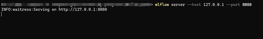
Next, let’s test if the MLflow UI is working properly. To start, you’ll need to launch the MLflow Tracking Server. Make sure to keep the command prompt open during the tutorial, as closing it will stop the server. Here’s the command you need to run in your terminal:

mlflow server --host 127.0.0.1 --port 8080

After running the above command, you will see the URL for the running MLflow UI displayed in the terminal, as shown in the image below.

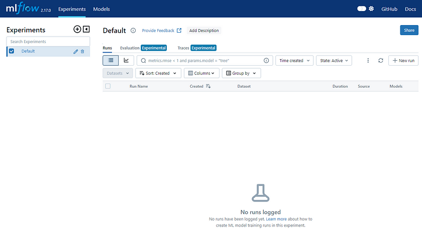
By opening this URL in your browser, you will see the UI as depicted in the following image:

MLflow Tutorial

In just a few minutes, this quickstart will guide you through key MLflow concepts, including how to log parameters, metrics, and models, the basics of using the MLflow fluent API, how to register a model during the logging process, how to navigate to the registered model in the MLflow UI, and how to load a logged model for inference.

Here, we use a simple example to train a model. This code primarily focuses on training and testing a Logistic Regression model using the Iris dataset, and calculating the accuracy of its predictions. The code loads the classic Iris dataset, a public dataset containing 150 flower samples, each with 4 features (sepal and petal lengths and widths), and divided into 3 categories: Setosa, Versicolor, and Virginica. The model predicts the flower category based on the 4 features (sepal length, sepal width, petal length, and petal width). Additionally, the code splits the dataset into training and test sets, with 80% of the data used for training (X_train and y_train) and 20% for testing (X_test and y_test).

Step 1: Set the Tracking Server URI

If you’re using a managed MLflow Tracking Server or if you’re running a local tracking server, ensure that you set the tracking server’s uri using:

import mlflow
mlflow.set_tracking_uri(uri="http://<host>:<port>")

Step 2: Train a model and prepare metadata for logging

In this section, we will log a model using MLflow. The steps include loading and preparing the Iris dataset, training a Logistic Regression model, evaluating its performance, and then preparing the model’s hyperparameters and metrics for logging.

import mlflow
from mlflow.models import infer_signature
import pandas as pd
from sklearn import datasets
from sklearn.model_selection import train_test_split
from sklearn.linear_model import LogisticRegression
from sklearn.metrics import accuracy_score, precision_score, recall_score, f1_score

# Load the Iris dataset
X, y = datasets.load_iris(return_X_y=True)
# Split the data into training and test sets
X_train, X_test, y_train, y_test = train_test_split(
    X, y, test_size=0.2, random_state=42
)
# Define the model hyperparameters
params = {
    "solver": "lbfgs",
    "max_iter": 1000,
    "multi_class": "auto",
    "random_state": 8888,
}
# Train the model
lr = LogisticRegression(**params)
lr.fit(X_train, y_train)
# Predict on the test set
y_pred = lr.predict(X_test)
# Calculate metrics
accuracy = accuracy_score(y_test, y_pred)

Step 3: Log the model and its metadata to MLflow

In the next step, we will log the trained model, the hyperparameters used for fitting the model, and the loss metrics calculated from evaluating its performance on the test data to MLflow. The process involves the following steps:

1. Initiate an MLflow run context to start a new run where we will log the model and related metadata.
2. Log the model’s parameters and performance metrics.
3. Tag the run for easy retrieval in the future.
4. Register the model in the MLflow Model Registry while saving the model.

# Set our tracking server uri for logging
mlflow.set_tracking_uri(uri="http://127.0.0.1:8080")

# Create a new MLflow Experiment
mlflow.set_experiment("MLflow Quickstart")
# Start an MLflow run
with mlflow.start_run():
    # Log the hyperparameters
    mlflow.log_params(params)
    # Log the loss metric
    mlflow.log_metric("accuracy", accuracy)
    # Set a tag that we can use to remind ourselves what this run was for
    mlflow.set_tag("Training Info", "Basic LR model for iris data")
    # Infer the model signature
    signature = infer_signature(X_train, lr.predict(X_train))
    # Log the model
    model_info = mlflow.sklearn.log_model(
        sk_model=lr,
        artifact_path="iris_model",
        signature=signature,
        input_example=X_train,
        registered_model_name="tracking-quickstart",
    )

The purpose of this code is to log the machine learning model’s training process, including the hyperparameters, performance metrics, and the model itself, and save this information using MLflow. It also registers the model in the MLflow Model Registry, allowing the model to be reused in different environments. This greatly facilitates the tracking of experimental results and the replication and deployment of the model in the future.

To view the results of our run, we can navigate to the MLflow UI. Since the Tracking Server is already running at http://localhost:8080, simply enter that URL in your browser.

Once the site opens, you’ll see a screen similar to the one below:

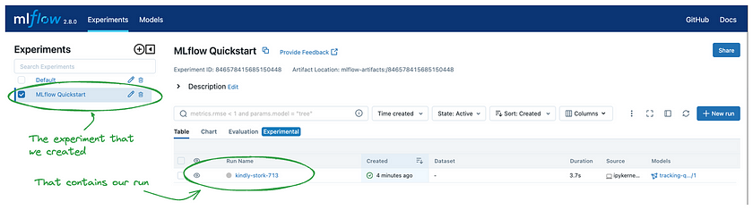
By clicking on the name of the experiment we created (“MLflow Quickstart”), you’ll be presented with a list of all the runs associated with that experiment. In the table view on the right, you’ll see a randomly generated name for the run.

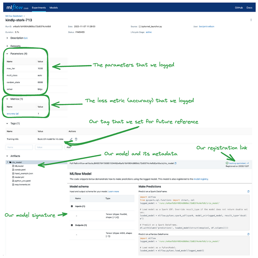
Clicking on the run’s name will take you to the run details page, where you can view all the information we’ve logged. The key elements are highlighted below to show how and where this data is displayed within the UI:

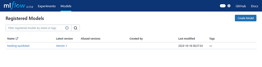
Our model has also been saved in the Registered Model section named “tracking-quickstart”:

Step 4: Load the model as a Python Function (pyfunc) and use it for inference

After logging the model, we can perform inference by:

1. Loading the model using MLflow’s pyfunc flavour.
2. Running predictions on new data with the loaded model.

# Load the model back for predictions as a generic Python Function model
loaded_model = mlflow.pyfunc.load_model(model_info.model_uri)

predictions = loaded_model.predict(X_test)
iris_feature_names = datasets.load_iris().feature_names
result = pd.DataFrame(X_test, columns=iris_feature_names)
result["actual_class"] = y_test
result["predicted_class"] = predictions
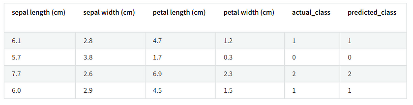
result[:4]

This code loads a previously saved model from MLflow and makes predictions on the test data. It then combines the actual labels of the test data with the predicted results into a table, displaying the first four rows. This allows us to verify the model’s performance on the test data and visually compare the predictions against the actual labels.

The output of this code will look something like this:

Of course, we can also specify the pre-trained model we want to run by selecting the run_id, and we can provide new data for it to make predictions. Below is a simple code example:

import mlflow.pyfunc
import numpy as np

# Set the MLflow Tracking URI to your server's address
mlflow.set_tracking_uri("http://127.0.0.1:8080")
# Load the model using the run ID logged in MLflow
run_id = "Your_run_id"  # Replace with the run ID found in the MLflow UI
model_uri = f"runs:/{run_id}/iris_model"
loaded_model = mlflow.pyfunc.load_model(model_uri)
# Define new test data
new_data = np.array([
    [5.1, 3.5, 1.4, 0.2],
    [6.7, 3.1, 4.7, 1.5]
])
# Use the loaded model to make predictions
predictions = loaded_model.predict(new_data)
# Print the prediction results
print("Predictions:", predictions)

In short, MLflow makes it convenient to train our models and save them for future use. When needed, we can easily load a previously trained model to run predictions, or even share it with others. Additionally, MLflow allows us to record detailed results from each training session, enabling effective version control of our models.

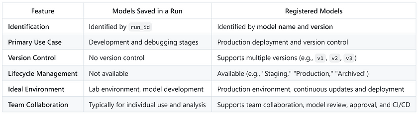
Differences Between Runs and Registered Models

Sometimes, we might wonder about the difference between a run and a Registered Model, especially since both can be used to load previously trained models.

• Run-based models: Best suited for development and experimentation, allowing for quick iteration and debugging.
• Registered Models: Ideal for production, offering version control and lifecycle management, making it easier to manage and update models in a team environment.

Key Differences Between the Two

If you want to use a registered model in a production environment, you can either register the model during training or register an existing model from a run as a Registered Model. For example:

mlflow.register_model(model_uri=f"runs:/{run_id}/iris_model", name="tracking-quickstart")

Here’s an example showing how to use registered models as loaded models:

import mlflow.pyfunc

# Load the model using the Registered Model name and version number
model_name = "your_registered_model_name"
model_version = 1  # Specify the version to load
model_uri = f"models:/{model_name}/{model_version}"
loaded_model = mlflow.pyfunc.load_model(model_uri)
# Use the model to make predictions
predictions = loaded_model.predict(new_data)

Conclusion

MLflow is a powerful platform that simplifies the management of machine learning projects, offering seamless integration for tracking experiments, saving models, and deploying them across various environments. By providing easy-to-use tools like the MLflow Tracking Server, Model Registry, and the flexible pyfunc interface, MLflow enables developers and data scientists to streamline the entire lifecycle of their models. Whether you are in the experimental phase or deploying models to production, MLflow’s robust features ensure that your workflow is organised, scalable, and reproducible. By leveraging MLflow, teams can efficiently manage models, track results, and collaborate more effectively, all while ensuring the scalability of machine learning efforts from development to production.

References

• MLflow Tutorial Page — Getting Started with MLflow Read me, accessed on 18 Oct, 2024. 2) MLflow Team — MLflow Tracking Quickstart Read me.